Project Metadata
Overview of the project context, scope, and tech choices.
Overview
- Role
- ML Engineer & Developer
- Client
- Academic Project
- Type
- Machine Learning Application
- Industry
- Computer Vision / Traffic Analysis
- Platform
- Web
- Duration
- -
Description
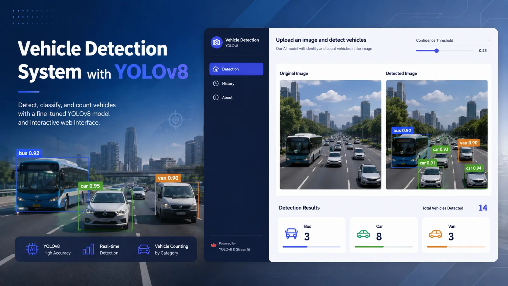
A web-based vehicle detection application using a fine-tuned YOLOv8 model to classify and count vehicles from uploaded images, with an interactive Streamlit interface for traffic analysis.
Key Features
- • Vehicle Detection & Classification
- • Confidence Threshold Adjustment
- • Side-by-side Comparison Visualization
- • Automatic Vehicle Counting by Category
- • Image Upload Interface
Tech Stack
Access
This project was my deliberate foray into computer vision, a domain I had only ever understood from a theoretical level. The driving question was straightforward: how accurately can a pre-trained object detection model perform on a specific use case like vehicle counting on real roads? And how much effort does it actually take to reach accuracy that’s genuinely useful in practice?
Context & Motivation
Conventional traffic analysis still relies heavily on inductive loop sensors embedded in the road surface or manual counting by field officers, both of which are expensive, inflexible, and provide no visual data. A computer vision-based approach offers a cheaper, more adaptable alternative: a camera and the right model are all you need.
I chose YOLOv8s (Small) by Ultralytics as the base model, a deliberate balance between inference speed and detection accuracy, making it well-suited for deployment on modest hardware while still hitting meaningful performance numbers.
Dataset
The dataset was sourced from Roboflow (vehicle-detection-vznzd-dkl8g, CC BY 4.0) and covers three vehicle classes: bus, car, and van. Intentionally limiting scope to three classes meant a cleaner, higher-quality annotation set. It’s better to have a tight, consistent dataset per class than a broad, noisy one.
The final dataset breakdown after splitting:
| Split | Images | Objects |
|---|---|---|
| Train | 9,218 | 18,494 |
| Valid | 287 | 427 |
| Test | 220 | 413 |
| Total | 9,725 | 19,334 |
Class distribution was expectedly skewed because cars dominate real-world traffic:
| Class | Count | Share |
|---|---|---|
| Car | 11,254 | 58.2% |
| Bus | 4,698 | 24.3% |
| Van | 3,382 | 17.5% |
Exploratory Data Analysis
Before training, I ran a thorough EDA pass to understand the dataset’s shape: distribution across splits, class balance, image size variance, and bounding box characteristics. A few findings worth noting:
- Image sizes are highly variable. Widths ranged from 180px to 1600px across train images (mean ~649px), which reinforces the need for a fixed
imgszresize during training. - Bounding box sizes vary widely too. Bus bounding boxes had areas ranging from 57 to over 1.5 million pixels², which is a natural consequence of having both close-range and distant shots in the same dataset.
- Van is the hardest class. It has the fewest examples (17.5% of total) and the widest size variance, which showed up clearly in final per-class metrics.
Fine-Tuning the Model
Training was done on Google Colab using a Tesla T4 GPU (15.8 GB VRAM). The pretrained yolov8s.pt weights were used as a starting point, overriding the original 80-class COCO head with a 3-class head.
from ultralytics import YOLO
model = YOLO('yolov8s.pt')  # Small: balance of speed and accuracy
results = model.train(    data='vehicle_dataset.yaml',    epochs=25,    imgsz=640,    batch=16,    device=0,  # Tesla T4    optimizer='SGD',    lr0=0.01,    momentum=0.937,    weight_decay=0.0005,    patience=15,    seed=42,)
Augmentation strategy was kept conservative but effective: horizontal flip (p=0.5), scale (±50%), translation (±10%), HSV jitter, and mosaic augmentation (p=1.0) through the first 15 epochs. Mosaic was disabled in the final 10 epochs (close_mosaic=10) to let the model stabilize on clean images before convergence.
Training completed in 1.2 hours across 25 epochs, producing an 11.1M-parameter fused model at 22.5 MB.
Model Performance
The best checkpoint (epoch 19, by mAP50-95) achieved:
| Metric | Score |
|---|---|
| mAP@50 | 0.8871 |
| mAP@50-95 | 0.7027 |
| Precision | 0.8182 |
| Recall | 0.8645 |
| F1-Score | 0.8407 |
Per-class mAP@50 breakdown shows the class-difficulty gradient clearly:
| Class | Precision | Recall | mAP@50 |
|---|---|---|---|
| Bus | 0.935 | 0.876 | 0.941 |
| Car | 0.897 | 0.832 | 0.922 |
| Van | 0.622 | 0.886 | 0.798 |
Bus and car performance is strong. Van underperforms on precision, a direct result of fewer training examples and higher visual similarity to both cars and buses depending on viewing angle. This is a known hard case in road datasets, and the mAP@50 of 0.798 is still usable for a proof of concept.
Inference speed on the T4 was 4.4ms per image, comfortably real-time capable.
Application Architecture
Streamlit was chosen as the UI layer for pragmatic reasons: Python end-to-end, zero frontend stack overhead, and simple local deployment. For a project centered on demonstrating an ML model, it hits exactly the right trade-off.
app.py │ ├── UI Layer (Streamlit) │ ├── File uploader (JPG/JPEG/PNG) │ ├── Confidence threshold slider (sidebar, default: 0.25) │ ├── Image info display (size, format, mode) │ ├── Two-column layout (original | detected) │ ├── Vehicle count badges (bus / car / van) │ └── Download button for annotated result │ ├── Detection Layer │ ├── load_model() → cached via @st.cache_resource │ └── detect_vehicles() → returns counts dict + annotated image │ └── State Layer (st.session_state) ├── annotated_image_bytes ├── original_image_bytes ├── vehicle_counts └── inference_errorModel caching was a critical optimization. Without @st.cache_resource, the model reloads on every UI interaction, causing a few-second delay each time. With caching, it loads once per session.
Session state was equally important. Streamlit reruns the entire script on every interaction, so without persisting results in st.session_state, the detection output would disappear the moment the user touched any other widget. Storing the annotated image as bytes and the count dictionary in session state keeps the results stable across reruns.
State is also reset cleanly when the user removes the uploaded file, ensuring no stale results from a previous image are shown with a new one.
Detection & Visualization Pipeline
The full image flow from upload to display:
- File uploaded via
st.file_uploader→ opened asPIL.Image, converted to RGB - PIL image passed to
detect_vehicles()as a NumPy array - YOLOv8s runs inference; bounding boxes drawn via
results[0].plot()(OpenCV internally) - Annotated image converted
BGR → RGB, then back to PIL, serialized to PNG bytes in memory - Both original and annotated images stored in
st.session_stateas bytes - Displayed side-by-side in two
st.columns; results persist across reruns
Vehicle counting is done directly from the detection results:
def detect_vehicles(image, model, conf_threshold):    if isinstance(image, Image.Image):        image = np.array(image)    results = model.predict(source=image, conf=conf_threshold, verbose=False)
    vehicle_counts = {'bus': 0, 'car': 0, 'van': 0}    for result in results:        for box in result.boxes:            class_name = model.names[int(box.cls[0])]            if class_name in vehicle_counts:                vehicle_counts[class_name] += 1
    annotated_image = cv2.cvtColor(results[0].plot(), cv2.COLOR_BGR2RGB)    return vehicle_counts, annotated_image
The confidence threshold defaults to 0.25, lower than the common 0.5 default, because real-world traffic images often include partially occluded or distant vehicles that don’t score highly but are genuine detections. Users can adjust this live via the sidebar slider; the detection result updates immediately on the next run.
The download button lets users save the annotated image directly, keeping the original filename prefixed with detected_.
Challenges & Learnings
The biggest challenge wasn’t in writing code, it was data quality. Images with poor lighting, heavily overlapping vehicles, or extreme camera angles significantly degraded detection accuracy. This made something very concrete: in ML projects, the majority of meaningful effort lives in data preparation, not in modeling.
Van detection was the hardest problem. Despite finishing with a usable mAP@50 of 0.798, precision on vans sat at 0.622, meaning nearly 4 in 10 van predictions were false positives. The root cause was twofold: the smallest class share (17.5% of objects), and visual ambiguity with cars from certain angles. Addressing this would require either more labeled van images or dedicated hard-negative mining.
Confidence threshold turned out to be a more important UX decision than I initially anticipated. I deliberately set the default to 0.25 rather than the common 0.5 because real-world traffic images often contain partially occluded or distant vehicles that won’t hit a high confidence score but are genuine detections. Exposing the threshold as a live sidebar slider, rather than hardcoding it, meaningfully increased the application’s utility across different input conditions and image qualities.
This project was my entry point into the ML ecosystem, and from here I understood that computer vision isn’t just about “calling a model API.” It’s about deeply understanding the trade-offs between accuracy, inference speed, data pipeline complexity, and the specific failure modes of your dataset.